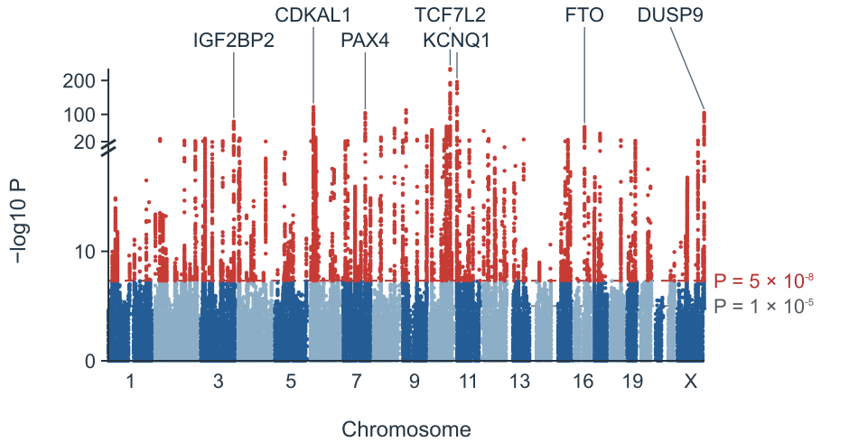
Type 2 diabetes GWAS
Association peaks across a type 2 diabetes GWAS.
Turn GWAS summary statistics into a Manhattan plot and QQ plot in your browser.
Explore association patterns across traits and species.
Association peaks across a type 2 diabetes GWAS.
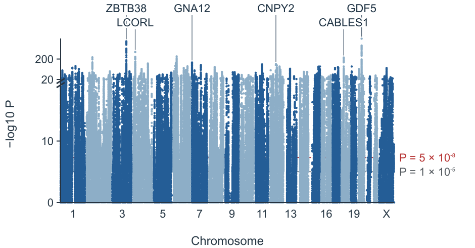
Dense association signals for adult height.
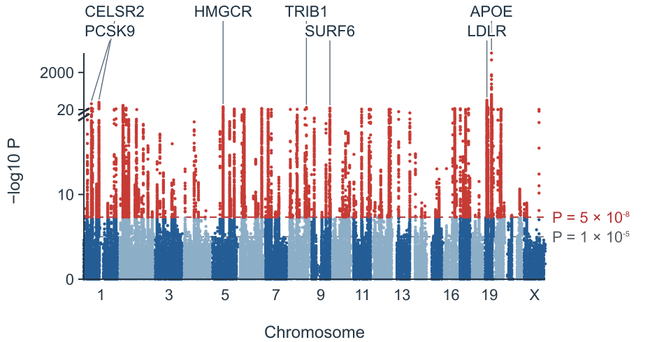
Lipid associations across the genome.
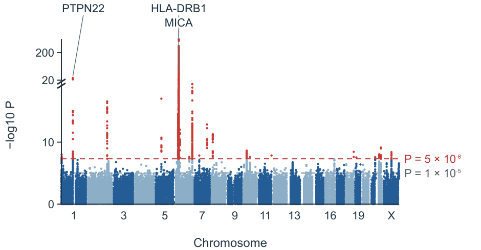
A prominent association in the HLA region.
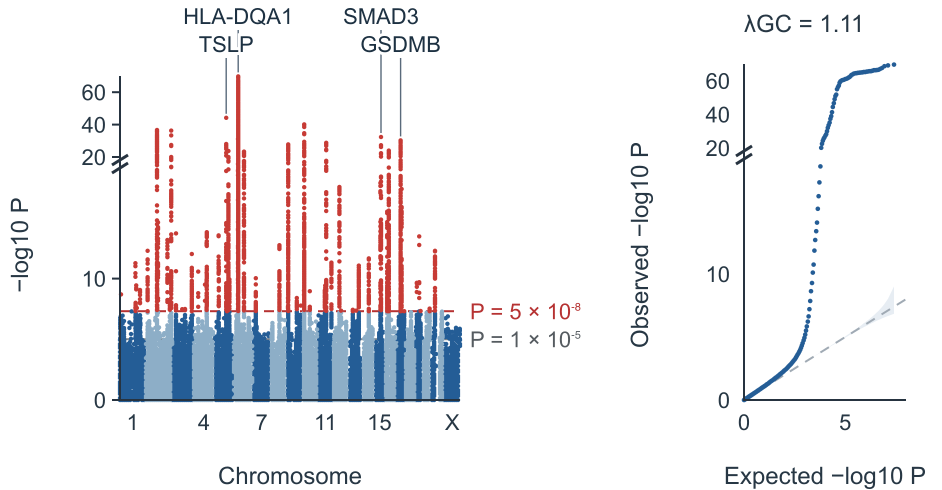
A Manhattan plot alongside its QQ plot.
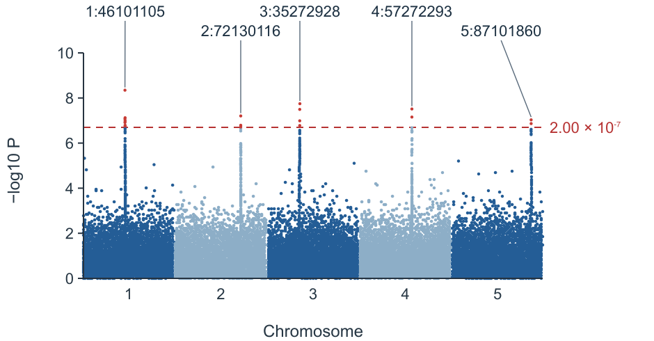
Five plant chromosomes with a Bonferroni threshold.
Import summary statistics and choose the display settings for your figure.
Import a GWAS summary statistics file or paste a small table.
Confirm chromosome, position, P value and optional variant ID columns.
Set the significance thresholds, locus window and labels.
Download a PNG or SVG, or export the loci table.
Common PLINK, REGENIE, SAIGE, BOLT-LMM, GEMMA, GAPIT, GWAS-SSF and METAL columns are recognized. Verify the mapping before plotting.
| Format | Chromosome | Position | P value | Variant ID |
|---|---|---|---|---|
| PLINK 1.9 | CHR | BP | P | SNP |
| PLINK 2 | CHROM | POS | P / LOG10_P | ID |
| REGENIE | CHROM | GENPOS | LOG10P | ID |
| SAIGE | CHR | POS | p.value | MarkerID |
| BOLT-LMM | CHR | BP | P_BOLT_LMM | SNP |
| GEMMA | chr | ps | p_wald | rs |
| GAPIT / TASSEL | Chromosome | Position | P.value | SNP |
| GWAS-SSF | chromosome | base_pair_location | p_value / neg_log_10_p_value | rsid / variant_id |
| PheWeb / FinnGen | chrom | pos | pval / mlogp | rsids |
| METAL | — | — | P-value | MarkerName |
| MAGMA / EWAS | CHR | START / MAPINFO | P | GENE / CpG |
References: REGENIE documentation · GWAS-SSF specification
Each point represents a variant. Chromosomes run along the horizontal axis and stronger associations appear higher on the vertical axis. Peaks can contain many correlated variants.

The conventional human GWAS threshold is 5 × 10⁻⁸; 1 × 10⁻⁵ is a suggestive threshold. Bonferroni uses 0.05 divided by the number of plotted variants.
| Genome-wide | 5 × 10⁻⁸ |
|---|---|
| Suggestive | 1 × 10⁻⁵ |
| Bonferroni | 0.05 / m |
References: Pe’er et al. 2008 · Turner 2018
A GWAS QQ plot compares observed P values with their expected distribution. The genomic inflation factor is the median observed χ² statistic divided by its null median; population structure and polygenicity can both increase it.
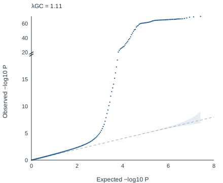
References: Devlin & Roeder 1999 · Bulik-Sullivan et al. 2015
A Manhattan plot shows each variant by genomic position and −log10 P value. Peaks identify regions associated with a trait.
Use qqman::manhattan(gwasResults, chr = "CHR", bp = "BP", p = "P", snp = "SNP"). This tool uses similar columns without requiring code.
Yes. Files are read in your browser without upload, up to 30 million rows. Overlapping background points are thinned; significant points are retained.
It approximates a Bonferroni correction for one million independent tests. Other species and study designs may need a different threshold.
λGC compares the median observed χ² statistic with its null expectation. There is no universal cutoff: polygenicity and large samples can raise it as well as population structure.
A lead is the most significant variant in a distance window, 500 kb on each side by default. This is not LD clumping and does not use a reference panel.
Yes. Select a human genome version and nearest-gene labels. For example, rs7903146 is at chr10:114758349 in GRCh37 and chr10:112998590 in GRCh38. The closest protein-coding gene is a positional annotation, not proof of a causal gene.
No. This tool makes Manhattan and QQ plots; it does not make Miami plots or LD-colored regional association plots such as LocusZoom.
Turn your summary statistics into a figure and locus table.
Make your Manhattan plot