Stopping distance against speed
Pick each point from a scatter plot of speed and stopping distance.
Source: R datasets (cars)
Upload a graph image, mark two values on each axis, and click points to extract their data.
| Dataset | X | Y |
|---|---|---|
| cars | 3.99 | 2.0 |
| cars | 3.99 | 10.0 |
| cars | 7.00 | 4.0 |
| cars | 7.00 | 22.0 |
| cars | 8.00 | 16.0 |
| cars | 8.99 | 10.0 |
| cars | 10.00 | 18.0 |
| cars | 10.00 | 26.0 |
| cars | 10.00 | 34.0 |
| cars | 11.01 | 17.0 |
| cars | 11.01 | 28.0 |
| cars | 12.00 | 14.0 |
| cars | 12.00 | 20.0 |
| cars | 12.00 | 24.0 |
| cars | 12.00 | 28.0 |
| cars | 13.00 | 26.0 |
| cars | 13.00 | 34.0 |
| cars | 13.00 | 34.0 |
| cars | 13.00 | 46.0 |
| cars | 13.99 | 26.0 |
| cars | 13.99 | 36.0 |
| cars | 13.99 | 60.0 |
| cars | 13.99 | 80.0 |
| cars | 15.00 | 20.0 |
| cars | 15.00 | 26.0 |
| cars | 15.00 | 54.0 |
| cars | 16.01 | 32.0 |
| cars | 16.01 | 40.0 |
| cars | 17.00 | 32.0 |
| cars | 17.00 | 40.0 |
| cars | 17.00 | 50.0 |
| cars | 18.00 | 42.0 |
| cars | 18.00 | 56.0 |
| cars | 18.00 | 76.0 |
| cars | 18.00 | 84.0 |
| cars | 18.99 | 36.0 |
| cars | 18.99 | 46.0 |
| cars | 18.99 | 68.0 |
| cars | 20.00 | 32.0 |
| cars | 20.00 | 48.0 |
| cars | 20.00 | 52.0 |
| cars | 20.00 | 56.0 |
| cars | 20.00 | 64.0 |
| cars | 22.00 | 66.0 |
| cars | 23.00 | 54.0 |
| cars | 23.99 | 70.0 |
| cars | 23.99 | 92.0 |
| cars | 23.99 | 93.1 |
| cars | 23.99 | 120.0 |
| cars | 25.00 | 85.0 |
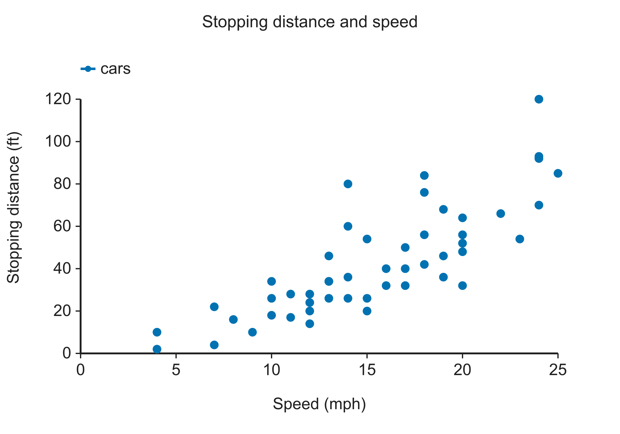
Pick each point from a scatter plot of speed and stopping distance.
Source: R datasets (cars)
Digitize group means and error-bar caps.
Source: R datasets (ToothGrowth)
Compare treated and untreated reaction rates.
Source: R datasets (Puromycin)
Trace survival curves from patient data.
Source: R survival (lung)
Extract a line from annual observations.
Source: R datasets (Nile)
A tilted, scanned figure — four-point calibration corrects the rotation.
Source: R datasets (ChickWeight)
Add an image to the plot digitizer by choosing a file, dropping it on the workspace or pasting a screenshot.
Click two known positions on each axis and enter their values.
Click points manually or pick a color and extract a curve or markers.
Review the points and export a CSV or copy a tab-separated table.
1To extract data from a figure, first calibrate its axes using known values.
2The plot digitizer shows per-pixel resolution; image resolution and click placement limit precision.
3For bars, distinguish the bar top from error-bar caps and consult the original caption before interpreting them.
Record the source figure and check extracted coordinates independently. Digitized Kaplan–Meier coordinates can support reconstruction methods such as Guyot et al. (2012).
Accuracy depends on image resolution and calibration. Check the displayed per-pixel resolution and compare repeated extractions. Drevon and colleagues studied the reliability and validity of digitized graph data. Drevon et al. (2017).
Yes. In the plot digitizer, select Log10 independently for each axis and enter positive calibration values.
Select Bar chart, calibrate Y, and click the bar top and error-bar caps. Consult the original caption to determine whether the bars represent SD, SEM, or confidence intervals.
Yes. Pick a color and use Line or Markers; overlapping or similarly colored marks may require manual correction.
Take a screenshot or copy the image and paste it here. Enlarge a vector figure before taking the screenshot for better resolution.
No. The plot digitizer processes images in your browser and does not upload them.
WebPlotDigitizer supports additional graph types. This page focuses on XY and bar graphs, log axes and examples with source data.
Report the plot digitizer used and the source figure, and describe how you checked the extracted coordinates.
Extract coordinates with the plot digitizer and download a CSV.